24 October 2019

By Shuai Zheng
R&D Division, Hitachi America, Ltd.
In the manufacturing industry, a factory receives production job orders from customers, starts processing job orders, and finally delivers products to customers. There are costs in this process sequence. Each job comes with a due time. Past-due cost is the cost when a job cannot be delivered on time. Inventory cost is the storage cost when the job is finished before due time and stays in factory. It is obvious that all manufacturing managers want on-time delivery and minimum past-due cost and inventory cost. However, achieving these goals requires an efficient dispatching rule. A dispatching rule is used to select the next job to be processed from a set of jobs awaiting service. This article describes work being conducted at Hitachi America’s R&D Division focusing on dynamic dispatching for due date-based objective where we proposed a reinforcement learning based approach for this problem.
In reinforcement learning, an agent interacts with an environment over many discrete time steps. At each time step t, the agent receives a state and performs an action following a policy. The agent receives a reward for this action and a new state is then presented to the agent. The policy will guide the agent’s action to maximize the reward that the agent receives. The cumulative discounted reward from time t is defined as:
,
where is a discount factor. We formulate dynamic dispatching problems using reinforcement learning elements. Figure 1 shows the overall design of this work. In the figure, environment includes job queue block and processing machine block. Machine block can include one processing unit or multiple processing units. There are many jobs waiting in job queue block to be processed. Agent is a reinforcement learning module. At each time step, reinforcement learning agent observes a state , which includes job queue state and machine state, then outputs an action using a deep learning model as function approximator. The agent also receives a reward from the environment for this action.
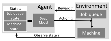
Figure 1: Manufacturing Dispatching using Reinforcement Learning
Job queue block can be further divided into two parts: job slot and backlog slot. We assume there are job slots and backlog slots. Each job has a processing time (job length) and a due time . Job arrives randomly. When a job arrives, it will be placed on one of the job slots randomly. If job slots are full, the job will be placed on backlog slots. Let indicate current time. Slack time of a job is defined as:
.
If , it means that if this job is started now, it will be completed before its due time; if , it means that it will be completed after its due time. We can now explain the design details of this system elements: state space, action space, and reward.
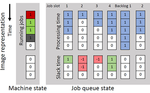
Figure 2: A state representation example: this state looks T=5-time steps ahead of current time and slack time array length is Z=3; there are n=4 job slots and m=10 backlog slots. The machine state tells that the next 4-time steps have been scheduled. For the job in job slot 1, p=3, slack = 1; for the job in job slot 3, p=2, slack = -1. There are 8 jobs waiting in backlog.
State space. State space includes both states of the machine and job queue. At any time step, we consider the states time steps ahead and we use a length array to represent the slack time. We use a 2-D matrix to represent machine state and job queue state. One example is shown in Figure 2. Value 1 in machine state means that the machine at that time step has been allocated, and value 0 means that the machine will be idle. Job queue state consists of job slots and backlog. Each job slot is represented using two arrays: processing time and slack time. The processing time array is represented using a length array, with the number of 1s indicating job length . The slack time is represented using a length array, where 1 means positive and -1 means negative . The sum of slack time array represents job . Backlog state is represented by several -length array, with a total of slots, where each slot represents a job. In Figure 2, backlog is represented using two 5-length array and there are 8 jobs in backlog.
Reward. Dispatching performance can be evaluated in terms of lateness , tardiness . Let the completion time of a job be . Lateness is the absolute difference between job due time and job completion time:
,
where . Tardiness only considers the lateness when the job is late. Thus, tardiness is defined as:
,
where . The objective of dispatching policy is to minimize the average lateness and tardiness.
There are many different factories and each factory has multiple similar product lines. It is not feasible to train and maintain a reinforcement learning module for each product line. We propose an approach to transfer policy between different manufacturing dispatching environments.
Given some random source states random target states we first find two projections by minimizing the objective function:
.
are similarity matrices for source environment and target environment respectively. is the similarity matrix between source and target environments. The state projection from source state to target state can then be given:
.
A source environment state can then be transferred to a target environment state using equation:
.
Suppose we have an optimal policy for source environment now. Using the computed , we can recover the policy in target environment by following the optimal states and actions from source environment.
We compared the proposed Deep Manufacturing Dispatching (DMD) with 7 other dispatching policies: 2 due time related manual designed rules (EDF for Earliest-Due-First, LST for Least-Slack-Time), 3 hyper-heuristics using machine learning (random forest, SVM, and neural network with 2 hidden layers), and reinforcement learning based RL-Mao and Tetris. Table 1 and 2 show that DMD gets the highest reward using lateness and tardiness under different trajectory length and job characteristics.
Table 1. Total discounted reward using different objective and trajectory length.
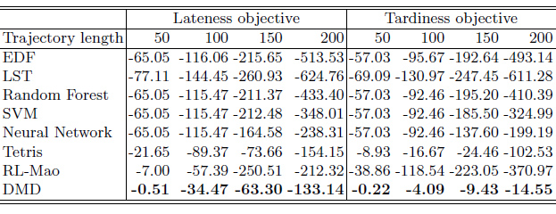
Table 2. Total discounted lateness reward with various job characteristics.
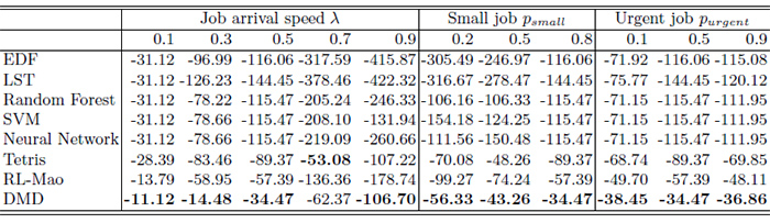
Figure 3 shows that policy transferring reduces training time and gives larger total discounted reward compared to training from scratch.
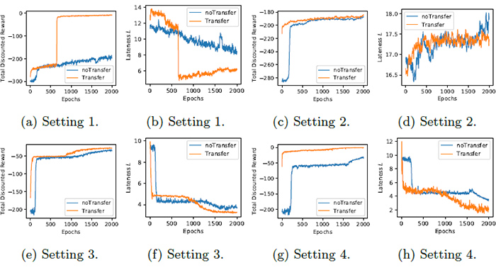
Figure 3: Policy transfer evaluation using Deep Manufacturing Dispatching
Enlarge (Open new window)
For more details on this work, please refer to our ECML/PKDD 2019 paper [1].
References