23 March 2021

Masayoshi Mase
Research & Development Group, Hitachi, Ltd.
As AI prediction models continue to make increasingly accurate predictions, there is growing demand to apply them to mission critical tasks such as credit screening, crime prediction, fire risk assessment, and emergency medicine demand prediction. For such applications, recent complex prediction models are often criticized as black boxes as it is difficult to understand why the prediction model produces a given output. Explainable AI (XAI) has been intensively studied to resolve this dilemma, and ensure transparency. Post-hoc explanation methods such as LIME [1] and SHAP [2] has been proposed for explaining which input variables are important. The Shapley value [3] from cooperative game theory is gaining popularity for the explanation. It has a mathematically reasonable definition for globally consistent local explanation, and widely used, especially for tabular data. However, conventional Shapley based methods are potentially evaluating unlikely or even logically impossible synthetic data points where the machine learning prediction might be unreliable. Our cohort Shapley uses observed data points only. It realizes reliable explanations that matches human intuition.
Shapley value [3] is used in cooperative game theory to define a fair allocation of rewards to a team of players that has cooperated to produce a value. Lloyd Shapley introduced it in his 1953 paper. The Shapley value is the unique method that satisfies the following four properties:
To understand black box predictions, we can see that each input variable is each player, and the predicted value is the produced value of the game. The problem then is how do we define the partial participation of input variables for the prediction.
Conventional baseline Shapley [4] (Figure 1) defines the partial participation of input variables by changing the input value and predicting on these synthetic data points. For example, when explaining the target subject (x1,x2,x3 ), it uses a baseline input (z1,z2,z3) as all absent, then the presence of the 1st input variable is defined as predicted values when the 1st variable is changed to the value of the resulting target subject (x1,z2,z3), and so on. Then we apply the Shapley value to the prediction on the synthetic data points. The process is potentially creating unlikely or even logically impossible combinations where the prediction model is likely to generate unreliable output.
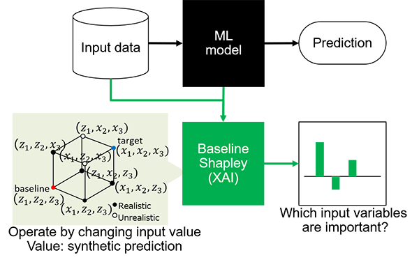
Figure 1: Illustration of baseline Shapley usage. Baseline Shapley uses input data and model to generate synthetic prediction by changing input value to apply Shapley value.
Our cohort Shapley (Figure 2) uses only observed data points and their predicted values. It operates by including and excluding data subjects. Here, all absence, or baseline cohort consists of all data points, then the presence of the 1st variable is defined as a prediction average of data points where the value of the 1st variable is similar to the 1st variable of the target subject x_1, and so on. We then apply the Shapley value to the cohort prediction averages. The process does not create synthetic data points.
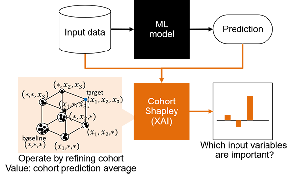
Figure 2: Illustration of cohort Shapley usage. Cohort Shapley uses input data and their predictions to calculate cohort prediction averages by refining cohort with similarity.
Here is an example on a popular Boston housing data set. Figure 1 shows cohort Shapley (CS) and baseline Shapley (BS) values for this target subject. As in the figure, baseline and cohort Shapley values are very different.
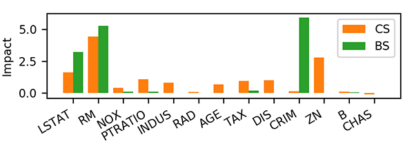
Figure 3: Baseline and cohort Shapley value for 205th subject of Boston housing data set. The baseline point is sample average in baseline Shapley.
In baseline Shapley ‘CRIM’, for example, was the most important variable, while in cohort Shapley it is one of the least important variables. We think that the explanation can be found in the way the baseline Shapley uses the synthetic data point at the upper orange cross in the left plot of Figure 4. The predicted value at the synthetic point is much smaller than that of the target subject. This leads to the impact of ‘CRIM’ being very high. Data like those synthetic points were not present in the training set and so the value represents an extrapolation where we do not expect a good prediction. We believe that an unreliable prediction there gives the extreme baseline Shapley value that we see for ‘CRIM’.
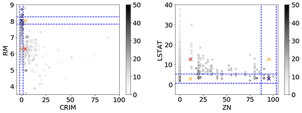
Figure 4: Two scatterplots of the Boston housing data. It marks the target (blue), baseline points (red), and synthetic points (orange) in baseline Shapley, depicts the cohort boundaries and shows predicted value in gray scale.
Baseline and cohort Shapley values have different characteristics. We should carefully consider about when and how to use these explanation methods. Especially, when a data set has dependence among input variables, we think that the cohort Shapley provides a more reliable and intuitive explanation. Also, cohort Shapley works with observed data points and their predicted values even if the target black box model itself is not available. This property looks favorable for auditing the model.
For more details, we encourage you to read our paper "Explaining black box decisions by Shapley cohort refinement."
This work was conducted in collaboration with Prof. Art B. Owen and Benjamin Seiler, Stanford University.