8 June 2022

Anjana G. Rajakumar
R&D Centre, Hitachi India Pvt. Ltd.
Water systems around the world are under tremendous stress to meet the growing water demand due to population growth, rapid urbanization, climate change, etc. Optimal water allocation and water distribution system control are essential for managing this water demand. Water demand predictions aid in these operations leading to sustainable management of water supply systems. These predictions help in system maintenance, expansion, and in planning daily network operations. They can also help in managing water network leaks.
In recent years, such predictions have also found wide application in near-optimal control operations of water networks. Water demand prediction is an active field, where different methods and techniques have been applied including conventional statistical methods and machine learning methods. Due to advancements in the field of sensing and IoT, an increasing amount of data is becoming available for water distribution systems, including water demand data. Therefore, we are seeing greater use of deep learning methods to develop models for water demand forecasting in recent years as deep learning methods can deal with seasonality as well as random patterns in the data, and provide accurate results compared to traditional methods.
In a study presented at EGU General Assembly 2021,[1] we looked at commonly used deep learning methods for the development of a short-term water demand forecast model for a real-world water system. This will help the water system operators and urban planners in choosing the right method to utilize for their work. The algorithms studied in this work were: (i) Multi-Layer Perceptron (MLP) (ii) Gated Recurrent Unit (GRU) (iii) Long Short-Term Memory (LSTM) (iv) Convolutional Neural Networks (CNN) and (v) the hybrid algorithm CNN-LSTM.
Hourly water demand data was obtained from a medium sized water network from Hillsborough County, Florida (USA). Data was available for 10 months from March 2012 to December 2012. The average system demand was about 113.68 MLD with a standard deviation of 33.92 MLD. Preliminary exploratory data analysis indicated presence of daily, weekly and monthly seasonality in this dataset. Auto Correlation Functions (ACF) were obtained to analyze the seasonality associated with the data.
Figure 1 shows the methodology adopted for this study.
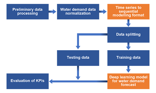
Figure 1. Study methodology
The core steps involved in the process are: (i) data normalization (ii) development of the sequence model/input data format (iii) defining the deep learning model architecture and (iv) model training and testing followed by evaluation. The latter step (step iv) is often carried out simultaneously with step (iii).
For the deep learning model, the length of the input size was varied from 2 to 14 data points. The equation below depicts the input-output data format used for the deep learning model, as in step (ii) of the methodology.
Qt=f(Qt-1,Qt-2,Qt-3 ,…,Qt-n)
In this equation, n is the size of input window in hours and Q denotes the flow (demand) in MLD, t denotes the timestep.
The output is the demand data for the current time step t. 75% of the data is used for training and the remaining for testing. The KPIs used for comparing these methods are Root Mean Squared Error (RMSE) value and Mean Absolute Percentage Error (MAPE).
As mentioned earlier, 5 different types of deep learning methods were used in this study. The hyperparameters were determined using grid search algorithm and all the models were implemented in python using Keras library. Adam optimization algorithm was adopted and MSE (Mean Squared Error) was used as the loss function for the weight and bias tuning.
It was observed that, the RMSE and MAPE values were minimal for values of n: 24 (1-day data as input). Also, it was observed that, CNN-LSTM performed better than other methods for demand forecast, followed by MLP. MAPE and RMSE values for the deep learning algorithms ranged from 5% to 25% and 9 to 20 MLD respectively. Figure 2 shows the actual and the predicted value (using CNN-LSTM) of demand for the test dataset for this analysis (RMSE: 9.952 MLD and MAPE: 6.776%).
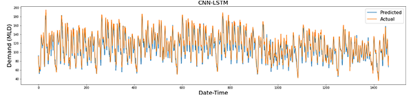
Figure 2. Actual and predicted demand
We observed that the frequency of data, amount of data, and quality of data has an impact on the deep learning model accuracy. In CNN-LSTM, CNN effectively extracts the inherent characteristics of historical water consumption data such as seasonality, and LSTM can fully reflect the long-term historical process and future trend. Hence, water demand forecast predictions using CNN-LSTM produced a better result when compared to other single models such as GRU, MLP, CNN and LSTM.
I’d like to acknowledge Avi Anthony Cornelio and N. Vinoth Kumar with whom this work was conducted and thank N. Vinoth Kumar for supporting the publication of this blog.